|
|
Post by Admin on Sept 15, 2023 21:27:13 GMT
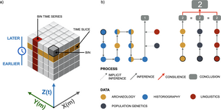 Fig 2. Graphical representations of selected methods: a) space-time cube model (after ESRI); b) comparison of two types of inference: On the left, data from different fields are compiled to draw a unified conclusion (analysis of Pohl’s [17] interpretation of our study region as an example), and on the right, consilience. doi.org/10.1371/journal.pone.0274687.g002The concept of the space-time cube is familiar to archaeologists. At its core, it is an application of the way we perceive (or have perceived in the past) archaeological excavations: In spatial quadrants and time phases. The quadrants in the xy grid are constant throughout the excavation, and the phases stack on top of each other, with the earliest at the bottom and the latest at the top. For our case study, we aggregated data into 5 km big (y dimension) and 25 years long (z dimension) hexagonal bins. The size of the hexagon was chosen as the largest in which the relevant processes can be observed; in Early Medieval archaeology, it roughly corresponds to the site catchment area of a single settlement, e.g., [45]. The time interval of 25 years was determined on the basis of the data properties. The time sensitivity of relevant archaeological dating is about half a century, i.e., ± 25 years. However, start and end dates can often be a quarter of a century, rarely as brief as decades or even years. The accuracy of our dates is therefore 50 years, but the precision is approximately 25 years. Accordingly, 25-year intervals were chosen for analysis, but the accuracy of the data requires that archaeological interpretation be limited to 50-year intervals. This method is very sensitive to the difference between no data (areas not analyzed) and null data (areas analyzed, but not found to contain any known sites). To account for this, we limited the space-time cube to the area used for data collection. Additionally, we excluded areas higher than 1,400 m above sea level (Fig 1: shades of brown). In our region, this altitude delineates the highest valley settlements from the lowest high-mountain pastures. The latter were excluded from the analysis because they are specialized seasonal settlements that were always dependent on valley settlements. |
|
|
|
Post by Admin on Sept 16, 2023 21:44:10 GMT
2.3. Time series clustering
Clustering is one of the most widely used machine learning techniques in the field of cultural heritage [39]. Its goal is to organize similar data into homogeneous groups or clusters. Clusters are formed by grouping objects that have maximum similarity with other objects within the cluster and minimum similarity with objects in other clusters. For large and complex data sets, unsupervised approaches offer the best solution. Time series clustering is a type of unsupervised clustering used for data with a temporal component [46, 47].
The concept of time- series clustering is deeply familiar to archaeologists having been used since the nineteenth century. At that time, for example, the three-age system, which divides the development of human civilization into the Stone Age, Bronze Age, and Iron Age, was defined by clustering similarly dated stone/bronze/iron artefacts. As most archaeologists know from experience, such clustering is relatively easy for a few artefacts or sites but becomes daunting when the numbers run into the hundreds or thousands of objects or sites. In such cases, unsupervised time series clustering can be used.
In this article, we applied time series clustering to classify sites into chronological groups. In each group, the chronology (start date, end date) of the sites is more similar to each other than that of the sites outside the group.
The similarity between the clusters is measured by the so-called “pseudo-F statistic.” The larger the pseudo-F value, the more different each cluster is from the other clusters [48]. There are several ways to calculate the pseudo-F statistic, each depending on which characteristics of the time series are considered important. In our experience, the most appropriate for archaeology is the "Profile (Fourier)" method, i.e., method based on Fourier series periodic function. It is used to cluster time series that have similar, smooth, and periodic patterns over time [42].
This method lends itself to the analysis of archaeological processes because they usually follow a consistent pattern: A gradually introduced innovation is followed by a peak of use and a steady decline. Thus, archaeological processes can be compared to seasons, where temperature follows a consistent annual pattern, with higher temperatures in summer and lower temperatures in winter. The “Profile (Fourier)” method is best suited to finding locations that have the most similar annual temperature patterns, for example, to distinguish between locations with mild and severe winters. A season in this example represents an archaeological phase or period.
In our case, we opted to ignore the range, i.e., the magnitude of the values in each period. To extend the analogy above, ignoring the range causes the change of seasons in two places occurring at the same times to be considered similar, even though the actual temperatures are different.
2.4. Modified emerging hot spot analysis
Spatial analysis is often called upon to determine the density of observed phenomena, and one of the most common tools to do this in archaeology is the so-called “hot spot analysis.” It uses the Getis-Ord G* statistic to calculate z-scores and p-values within a given spatial neighborhood. These indicate whether the observed spatial clustering of high and low values is more (hot spot) or less (cold spot) pronounced than would be expected from a random distribution, e.g., [49].
In this article, we have used an emerging hot spot analysis that examines the clustering of high and low values over time, in addition to spatial trends. The space-time cube is evaluated bin-by-bin, and each bin is analyzed relative to its space-time neighbors. Thus, each site is related not only spatially but also temporally to neighboring sites. The result is similar to the traditional hot spot analysis, except that it is in 3D (where the z dimension represents time).
Such a result can deliver an overwhelming amount of information. Therefore, the tool evaluates the trends of hot spots and cold spots over time using the Mann-Kendall trend test, e.g., [50] and categorizes each location in the study area accordingly. For example, a location is considered a consecutive hot spot if it has an uninterrupted series of statistically significant hot spot bins over the latest time step intervals, but less than 90% of the total [42]. The resulting 2D representation of trends can be termed a “trend map.”
However, the trend map provided by the tool is not suitable for archaeology for two reasons. First, it assumes that the latest records are the focus of analysis. Second, it was designed for data sets much larger than ours and those of most archaeological studies.
We therefore modified the trend map by focusing on chronological periods previously calculated by the time series clustering method. For example, a location was considered a first period consecutive hot spot if it had an uninterrupted hot spot series of at least 100 years within the first period (detailed description in S1 Table). We term this an “archaeological trend map”.
In emerging hot spot analysis, the spatial and temporal neighborhoods have a significant influence on the results. We found, through empirical observation, that the best results for hot spots and cold spots were obtained with different settings. For cold spots: fixed distance method with 20 km neighborhood, and time step three. For hot spots: k-nearest neighbors (kNN) method with six spatial neighbors, time step one [42].
Therefore, we have introduced another archaeology-specific modification to the tool. For the purposes of this article, we superimposed the cold spots derived using the first settings with the hot spots derived using the second settings in a single visualization. We refer to this method as “multiscale emerging hot spot analysis.”
To ensure the highest level of methodological transparency, reproducibility, and transparency and to reduce the time researchers spend replicating the work of other research groups, we provide the ready-to-re-use data in GIS format and the GIS protocol (S1 Appendix).
|
|
|
|
Post by Admin on Sept 17, 2023 20:52:24 GMT
3. Theory
3.1. Consilience
The specifics of archaeological inference, e.g., [51], are not often outlined in articles such as ours. In this case, however, it is necessary because academic passions on the question of the migration of the Slavs have long been running high, and the methods of inference are often scrutinized. Moreover, this topic is invariably interdisciplinary, but the interdisciplinarity is achieved through a variety of approaches.
In order to enrich this discussion with the most objective archaeological information possible, we have chosen to base our inference on consilience of induction. Consilience, also known as “convergence of evidence,” is a scientific principle that states that the same conclusion is much stronger when drawn from independent and unrelated sources. Confidence is strongest when evidence from different fields is considered because the methods and/or data are different [52].
Although it is rarely referred to by its name, this principle is popular in archaeology. For example, consilience is applied whenever radiocarbon dating is invoked to support archaeological dating.
It is important to distinguish between consilience, where conclusions are drawn independently before being correlated, and the more common interdisciplinary approach to the study of Slavic migrations, where data from different fields is compiled to draw a unified conclusion with a mix and match approach (Fig 2Bb). To this end, we have been careful to consider only information from each field that has not been influenced by findings from another field. For example, in the Discussion we consider linguistic information [53], but disregard the conclusions drawn on the same subject matter using supporting evidence from archaeology [54]. We also take care to include only interpretations reached by domain specialists, as reinterpretations by non-specialists can be problematic [6].
3.2. Material culture as ethnicity, identity, and habitus?
The main archaeological argument for the migrations of the Slavs is based on the association of the Slavs with various archaeological cultures or habitus. For instance, the archaeological assemblages of the so-called Prague Culture are associated with the Early Slavs, e.g., [55–61].
From a modern theoretical perspective, this argument draws on Pierre Bourdieu’s [62] notion of habitus; its basic premise is that practical knowledge is embodied in daily practices and that material culture, including pottery, expresses these practices, e.g., [63]. However, equating a habitus (e.g., the archaeological assemblages of Prague culture) with a people/tribe/ethnicity (e.g., the Early Slavs) is an additional step that Bourdieu did not anticipate. In much of the literature after the mid-1960s, the notion that material culture is more or less directly related to cognition of peoples was questioned by many; the acceptance that archaeological cultures simply cannot be directly correlated with ethnicity took hold, e.g., [64, 65].
Rather than engage in this discourse, we based our argument only on the categories of archaeological data that are indisputable: Location and chronology of the site. Our inference thus eclipses theoretical issues about the associations of material culture with ethnicity, e.g., [66], identity, e.g., [67], or habitus, e.g., [63]. Whether or not the Prague Culture archaeological assemblages are associated with the Early Slavs was immaterial to our conclusions.
|
|
|
|
Post by Admin on Sept 18, 2023 21:08:56 GMT
4. Results 4.1. Archaeological periodization The result of our time series clustering is the archaeological periodization of sites. The most archaeologically meaningful result is when the data is clustered into three periods (pseudo-F statistic value 421.595). These are the Late Antiquity and two Early Middle Ages periods (Fig 3). The latter two correspond to the traditional periodization of the jewelry into the Carantanian and the Köttlach phases, e.g., [68] or groups A/B and C of Eichert [69]. 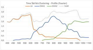 Fig 3. Archaeological periodization with time series clustering: LA—Period 1, Late Antiquity; EMA1—Period 2, Early Middle Ages 1; EMA2—Period 3, Early Middle Ages 2. Values on x axis are years CE, values on y axis are unitless and relative. doi.org/10.1371/journal.pone.0274687.g003Three important conclusions may be drawn from these results. The first is, that the general increase in sites between 400 and 500 CE and the decrease after 1000 CE does not reflect reality, as we know it from numerous sources, e.g., [22, 70]. Rather, it reveals the weakness of the underlying data set: The period before 500 CE has not been collated systematically, and data for the period after 1000 CE (which, until recently, was not considered relevant to archaeology in the region, e.g., [71]) is lacking. Regardless, the present data set is suitable for the study of the half millennium between 500 and 1000 CE, which was the aim. Second, unlike changes in material culture, changes in landscape are more gradual and often overlap. For example, the time series of Late Antiquity does not end until 1000 CE, as some sites exhibit continuity from Late Antiquity onward (for example, the town of Kranj, e.g., [72]). The results of time series analysis in archaeology are therefore complex and must be interpreted with great care. Third, we substantiated the long-established periodization of the Early Middle Ages into two periods by an independent source of data: The chronology of sites rather than the typology of jewelry. This, then, is the first quantitative evidence that changes in jewelry styles taking place in the second half of the 9th century were reflected in changes in the archaeological landscape. The most likely explanation is that both changes had the same underlying cause, which however is beyond the scope of this article. |
|
|
|
Post by Admin on Sept 19, 2023 20:56:14 GMT
4.2. Archaeological landscape The emerging hotspot analysis revealed an astonishing quantity and quality of information (Fig 4). Most relevant to our topic are the extensive areas of cold spots in the northern part of the region and the general patchiness, i.e. activity is concentrated in enclaves. In this respect, the archaeological landscape between 500 and 1000 CE differs from both the preceding Roman period settlement and subsequent High Medieval period, which both exhibit a more regular pattern of settlement. This is important in providing a context for understanding various historical processes. For example, the reason it is so difficult for historiographers to define the exact borders of Carniola, e.g., [3] and Carantania, e.g., [4] is that in the patchy landscape precise fixed borders most likely never existed. 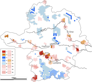 Fig 4. Archaeological trend map of the modified categorization of the multiscale emerging hot spot analysis. See S1 Table for the legend (authors E.L. and B.Š; contains information from OpenStreetMap and OpenStreetMap Foundation, which is made available under the Open Database License; contains information adapted and modified from Copernicus Land Monitoring Service product EU-DEM25, which was produced with funding by the European Union). The main focus of this article was migration. The two tools for detecting migrations in our data were provided by Curta [13]. First, migration must have occurred if settlements and cemeteries suddenly appear in a previously sparsely populated area, i.e. cold spots are immediately followed by hot spots. Second, migration can also be detected by the sudden appearance of a material culture without local traditions or parallels in a given area. With the first tool, migration was documented in the easternmost part of the study area. In the period between 450 and 500 CE this is a cold spot area, but after c. 500 CE hot spots appear along the river Mura (Ger. Mur). After a period of consolidation until c. 600 CE, a series of small-scale neighbourhood migrations upstream of the Mura and the adjacent Drava (Ger. Drau) rivers is documented by numerous hot spots (Fig 5A; S2 Appendix). |
|

