|
|
Post by Admin on Mar 21, 2018 19:04:24 GMT
 Relationship between BMI and Skeletal Robusticity Cross and Wright (2015) argue that Amelia Earhart is excluded because her physique was extremely linear and gracile, and therefore inconsistent with the skeletal remains which Hoodless assessed as belonging to a stocky individual. They argue, using height and weight (68 in. and 118 lb.) from her pilot’s license, that Earhart’s body mass index (BMI) is 17.9, placing her in the extreme lean range. From this they leap to infer a gracile skeleton that Hoodless would not have mistaken for that of a stocky male. There are two problems with this inference: (1) there is no necessary relationship between BMI and skeletal robusticity, and (2) available evidence does not support the inference that Earhart’s skeletal structure was gracile. I shall examine both of these in turn. The purpose of computing a BMI is to assess body fat, albeit an imperfect indicator. Since it is a ratio (weight/height2), all components of weight, including muscle and bone, in addition to fat, contribute to the value. Body proportions also play a role (Norgan 1994). On average, however, higher BMIs correspond to more body fat. But what does that say about skeletal robusticity? There are several lines of evidence suggesting that the relationship is not close.  The size of articular surfaces is one measure of bone robusticity. In the FDB data, using forensic height and weight to calculate BMI, the humerus and femur head diameters, femur epicondylar and tibia proximal breadths do not have significant correlations with BMI. Normalizing them by bone lengths increases the correlations slightly but they still do not reach statistical significance. Ding et al. (2005) measured proximal tibia articular surface area from MRI scans and compared it to BMI. The correlations were 0.25 and 0.16 for medial and lateral tibia articular surface areas, respectively. These correlations are statistically significant but so weak they lack predictive power. Joint surface size is likely a good indicator of lean body mass but has little to do with BMI. Femur head size has a moderately high correlation with weight and has been used to estimate weight in archeological samples (Auerbach & Ruff 2004), which would not normally have excessive fat. However, height is weakly correlated with weight, so the ratio of weight to height2 diminishes the relationship with skeletal robusticity. Another measure of robusticity is the size of the midshaft in relation to length, already discussed above concerning Hoodless’s sexing method. Femur midshaft robusticity has a moderate correlation with BMI in our forensic database, 0.46 for females and 0.44 for males, which is statistically significant but also too weak to discriminate robust from gracile skeletons using BMI. The problem of course is that neither Cross and Wright (2015) nor anyone else has any idea how Hoodless made the judgment that the skeleton was that of a stocky person. But what is clear is that the inference from BMI provides no basis to exclude the bones as belonging to Amelia Earhart, Hoodless’s assessment notwithstanding. |
|
|
|
Post by Admin on Mar 23, 2018 18:28:01 GMT
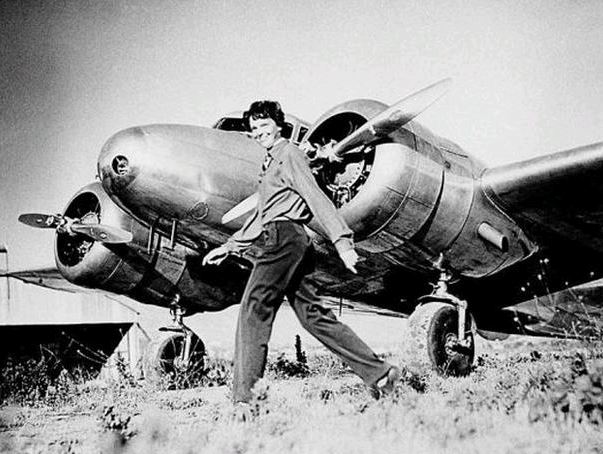
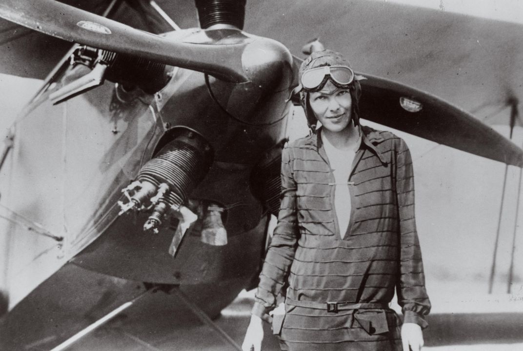
Amelia Earhart’s Body Build It is now possible to address the question of what Earhart’s body build actually was, since it bears on what Hoodless may have seen before him. Cross and Wright (2015) characterize Earhart as tall, slender, and gracile, citing numerous photos of her to support this assessment. However, the few photos showing Earhart’s bare arms or legs (Figure 5) show a woman with a healthy amount of body fat. The photos in Figure 5 are inconsistent with a weight of 118 pounds and a BMI of 17.9, which according to contemporary standards is in the underweight or undernourished category. If her height is actually 5'7", that brings her BMI to 18.5, just to the lower border of healthy weight. But even that is inconsistent with the photos in Figure 5. It is evident from Figure 5 that Earhart’s calves and ankles cannot be described as slender. In the 1933 photo she is standing next to a woman somewhat taller, but with rather more slender ankles. One of Earhart’s biographers, Susan Butler (1997), recounts that because of her thick ankles, her legs could be described as “piano legs.” Thick ankles are not normally due to an undesirable distribution of fat; the subcutaneous fat layer is normally thin, the ankle configuration owing to underlying bone and muscle (Weniger et al. 2004). Ankle circumference is often used as a measure of frame size (Callaway et al. 1991). Calf and ankle circumference are strongly correlated with weight (Cheverud et al. 1990a), the former reflecting mainly muscle and fat, the latter mainly bone. Empirical Estimation of Weight Weight can be estimated within reasonably tight limits if appropriate information is available. Circumferences typically have the highest correlation with weight. The extensive U.S. military anthropometric surveys provide the simple bivariate correlations of 259 variables (Cheverud et al. 1990a). These correlations and the means and standard deviations (Gordon et al. 1989) allow construction of a covariance matrix from which regression equations can be calculated. Waist circumference at the level of the umbilicus was used to estimate weight. It is above the rim of the pelvis and corresponds to the level at which the trousers were worn. Waist circumference obtained from Earhart’s trousers is 27.375 inches (69.53 cm). The average for U.S. military women is 79.2 cm, about 10 cm larger than Amelia Earhart’s measurement. This supports what is evident from the photographic record, that she had a narrow body. Table 4 shows estimates of Earhart’s weight using waist circumference and a height of 67 inches.  FIG. 5—Photos of Amelia Earhart showing body fat/body mass of arms and legs inconsistent with a weight of 118 pounds. Photos courtesy of Remember Amelia, the Larry C. Inman Historical Collection on Amelia Earhart. Waist circumference alone estimates Earhart’s weight at slightly more than the weight given on her pilot’s license, but with a large error. Including height raises the estimate 10 pounds, to 129.7, and reduces the error more than a kilogram. The 90% confidence interval (114.8–144.3) includes the weight on her pilot’s license, but it is equally likely that she weighed somewhat more than 130 pounds. Using a height of 67 inches and a weight of 130 pounds yields a BMI of 20.4, a normal value very much in keeping with the photographic evidence in Figure 5. The calf and ankle morphology may also suggest that her limb bones were not as gracile as supposed by Cross and Wright (2015) based on their assessment of her BMI. Unfortunately, we have only photographic and anecdotal evidence of Earhart’s ankle and calf size, but Butler’s (1997) characterization suggests that they exceeded those of most women of her height and weight. |
|
|
|
Post by Admin on Mar 25, 2018 18:44:28 GMT
Estimation of Humerus and Radius Length Among the many photos of Amelia Earhart is one showing her standing with right arm fully extended holding a can of Mobile Lubricant (Figure 6). An exemplar of the can was obtained by Jeff Glickman of Photek. A known dimension of the oil can provides a scale allowing the pixel coordinates of points on Earhart’s arm to be converted to linear distances (Glickman 2017). The major difficulty is identifying osteological points underlying the soft tissue. Figure 6 shows the locations for proximal and distal humerus and radius estimated to correspond to measuring points on dry bones. It is not possible to locate these points exactly, but they should provide reasonable approximations. The points shown in Figure 6 yield a humerus length of 321.1 mm and a radius length of 243.7 mm, compared to 325 and 245 for the corresponding Nikumaroro bones. The brachial index obtained from these estimate is 75.9, which compares favorably to the 76 obtained by Glickman on a different photograph (Glickman 2016b) Estimation of Tibia Length Estimating Amelia Earhart’s tibia length is more problematic than the radius and humerus because we have not identified a photo showing her lower leg allowing identification of osteological points and a scalable object. Therefore, two regression methods have been used: (1) estimating from stature and (2) estimating from inseam length of Earhart’s trousers. Estimating from stature is straightforward and was accomplished by regressing tibia length on stature using females from our database. The equation is: Tibia length = 2.1601 (height) + 4.8335 ± 12.50 Substituting Glickman’s measured height of 67 inches (170.18 cm) into the equation yields a point estimate of 372.4 mm.  FIG. 6—Amelia Earhart with right arm extended and points marked where humerus head, distal humerus, proximal radius and distal radius were located. Photo courtesy of Purdue Special Collections, Amelia Earhart Papers, George Putnam Collection. Estimating from inseam length is less straightforward and involves using regression equations from U.S. military anthropometric data. Unfortunately, a direct measurement of tibia length is not included in the military data. The two dimensions most closely approximating my needs are crotch height and lateral femur epicondyle height. The procedure is as follows: 1. Adjust inseam length to crotch height by adding ankle height. This assumes that Earhart’s trouser legs were level with the sphyrion landmark, the tip of the fibula. Earhart’s inseam measurement is 28.625 inches, or 727 mm. The ankle height adjustment, obtained from Cheverud et al. (1990b), is 63 mm, making Earhart’s crotch height = 727 + 63 = 790 mm. 2. Estimate Earhart’s lateral femur condyle height using regression equation in Cheverud et al. (1990b:780). The equation is: Lateral femur epicondyle height = 0.526 (crotch height) + 55.195 ± 8.53 Substituting 790 mm yields a point estimate of 470.7 mm. 3. Adjust lateral femur condyle height to tibia length by subtracting ankle height (63 mm, as above) and femur distal condyle height, 36 mm (Simmons et al. 1990). The point estimate is 470.7 − 63 − 36 = 371.7. There are admittedly several adjustments involved in this process, but they are all reasonable. Most of the variation in lateral condyle height involves tibia length, so minor variation in adjustments will not have major influence on the estimate. Crotch height has a much higher correlation with femur lateral condyle height, and hence with tibia length, than height. However, the estimates from height and lateral femur condyle height are very similar, 372.4 versus 371.7, so I will take 372 mm as the estimate of Earhart’s tibia length. |
|
|
|
Post by Admin on Mar 28, 2018 18:44:01 GMT
 Do the Nikumaroro Bones Fit Amelia Earhart? When confronted with human remains of unknown origin, the procedure followed in ordinary forensic practice is to develop a biological profile, and from among missing persons, select those that fit the profile. At that point one attempts to make a positive identification by using features seen on the bones that can also be seen in premortem records of the possible victims. The premortem records may consist of dental or frontal sinus images, or increasingly, DNA taken from remains and comparing to the victim or relatives of the victim. A positive identification is made when premortem features match the victim and have a low probability of matching anyone else. In the case of the Nikumaroro bones, the only documented person to whom they may belong is Amelia Earhart. Her navigator, Fred Noonan, can be reliably excluded on the basis of height. His height was 6'1/4", documented from his 1918 Seaman’s Certificate of American Citizenship. I made nine stature estimates of the Nikumaroro bones, three each for the humerus, radius, and tibia, using male equations in Fordisc for 19th-century males, WW2 males, and 20th-century males. Noonan’s height falls outside the 90% confidence intervals for all nine estimates, and outside the 95% for five of the nine estimates. It is clear that the Nikumaroro bones are unlikely to have belonged to Noonan. Eleven men were killed at Nikumaroro in the 1929 wreck of the Norwich City on the island’s western reef, something over four miles from where the bones were found in 1940.5 This number included two British and five Yemeni that were unaccounted for, but we have no documentation on them and there is no evidence that any survived to die as a castaway. The woman’s shoe and the American sextant box are not artifacts likely to have been associated with a survivor of the Norwich City wreck. If an Islander somehow ended up as a castaway, there is likewise no evidence of this.  FIG. 7—Histograms of 2,777 Mahalanobis distances (D) from the Nikumaroro bones, by sex. The line shows Earhart’s position in the distribution. If the skeleton were available, it would presumably be a relatively straightforward task to make a positive identification, or a definitive exclusion. Unfortunately, all we have are the meager data in Hoodless’s report and a premortem record gleaned from photographs and clothing. From the information available, we can at least provide an assessment of how well the bones fit what we can reconstruct of Amelia Earhart. Because the reconstructions are now quantitative, probabilities can also be estimated. Estimates of humerus, radius, and tibia lengths obtained from Amelia Earhart allow one to proceed as one normally would in a forensic situation. The Nikumaroro remains can now be compared to Amelia Earhart to address the question of whether she can be excluded or included. It is already apparent that Earhart’s vector of measurements, [321.1,243.7,372] is similar to that of the Nikumaroro bones [325,245,372]. These vectors contain both size and shape information, so a comparison should capture both of those elements. This was accomplished by computing Mahalanobis distance (D) of 2,776 individuals in our postcranial database from the Nikumaroro bones. Amelia Earhart’s data were included to yield N = 2,777. Figure 7 displays a histogram of the distances, by sex, of 2,777 individuals from the Nikumaroro bones. The vertical line shows Earhart’s position in the two distributions. She is clearly in the left tail of both distributions, but more so for females. Her z-score in the female distribution is − 2.38 (p = 0.017) and in the male distribution − 1.87 (p = 0.061). She has a low probability of coming from the male distribution and a much lower one for the female distribution. Earhart is in the first bin of the histogram for females, along with only two other females (0.526%). There are 16 males in the first bin (0.725%) One might argue that if the Nikumaroro bones are actually those of Amelia Earhart, the distance should be zero, but that expectation is unrealistic for at least two reasons: (1) it would require that my estimates of bone lengths were made without error, which is highly unlikely, and (2) it would require that Hoodless measured the Nikumaroro bones without error, which is also unlikely. |
|
|
|
Post by Admin on Mar 30, 2018 18:46:11 GMT
 It should be mentioned that a sample of Micronesian or Polynesian bone measurements was unavailable to test against the Nikumaroro bones. I consider it highly unlikely that inclusion of such a sample would have changed anything. As Figure 3 shows, the Nikumaroro bones are more similar to Euro-Americans than they are Micronesians or Polynesians, which suggests they would produce even fewer nearest neighbors. Another approach to the question is to examine Earhart’s rank in the distributions. For clarity, I should point out that if any individual in our sample had a vector of measurements identical to the Nikumaroro bones, the distance would be zero and have a rank of one, that is, most similar to the Nikumaroro bones. But not one from our 2,776 individuals had a vector identical to Nikumaroro’s. The lowest Mahalanobis distance is 0.12599, resulting from a vector of [322,243,369]. That vector is noteworthy because its elements are uniformly shorter than Nikumaroro, 3 mm for humerus and tibia and 2 mm for radius. Hence the most similar individual is almost identical in shape but differs slightly in size. The largest distance is 4.57, from a vector of [361,252,430]. It is larger than Nikumaroro in all dimensions, but shape still dominates because the differences range from only 9 mm (radius) to 58 mm (tibia). These examples suggest that the particular combination of bone lengths has considerable power to individualize. Earhart’s rank is 19, meaning that 2,758 (99.28%) individuals have a greater distance from the Nikumaroro bones than Earhart, but only 18 (0.65%) have a smaller distance. The rank is subject to sampling variation, so I conducted 1,000 bootstraps of the 2,776 distances, omitting Earhart, then replacing her to determine her rank. Her rank ranged from 9 to 34, the 95% confidence intervals ranging from 12 to 29. If we take the maximum rank resulting from 1,000 bootstraps, 98.77% of the distances are greater and only 1.19% are smaller. If these numbers are converted to likelihood ratios as described by Gardner and Greiner (2006), one obtains 154 using her rank as 19, or 84 using the maximum bootstrap rank of 34. The likelihood ratios mean that the Nikumaroro bones are at least 84 times more likely to belong to Amelia Earhart than to a random individual who ended up on the island.  The Gardener and Greiner method requires intervalizing a continuous distribution. The above procedure dichotomized the distribution, breaking it at Earhart’s rank, and at the maximum bootstrap rank. It might be argued that this weights the result in favor of similarity of Earhart to the Nikumaroro bones. Even if one breaks the distribution into deciles, the likelihood ratio is still 10. Regardless of how one chooses to break the distribution, the fact remains that Earhart is more similar to the Nikumaroro bones than all but a small fraction of random individuals. The above analysis considers only the comparison of Earhart to the Nikumaroro bones in relation to every other distance from Nikumaroro in our database. A more robust distribution of distances can be obtained by randomly sampling individuals from the database and comparing them to the sample as described above. Each randomly sampled individual serves as an unknown in the same manner as the Nikumaroro bones in the previous analysis. I randomly sampled 500 individuals from the database, omitting each randomly sampled individual in turn from the comparison because it would obviously have zero distance from itself. Sex was ignored for this exercise. From the 500 randomly sampled individuals, 17 had zero distance from another individual, that is, had an identical vector of measurements. One had an identical vector with two individuals, giving a total of 19 identical vectors from the 500 random samples, or 3.8%. This illustrates that identical vectors are a comparatively rare event. Summary statistics of the means, standard deviations, minima and maxima obtained from the 500 random samples are shown in Table 5. The summary statistics of the Nikumaroro bones are included for comparison. The data in Table 5 reveal that the entire 500 randomly sampled individuals have limited similarity to any other bones in the sample. The mean of the 500 means (2.2268) is somewhat higher than that for the Nikumaroro comparison, and the average minimum (0.1681) is also higher than the Nikumaroro comparison. But the Nikumaroro statistics are within the range of the 500 randomly sampled individuals. That the Nikumaroro comparison has somewhat lower distances only means that the Nikumaroro bones are closer to the average than many of the randomly sampled individuals. |
|

