|
|
Post by Admin on Jan 11, 2019 18:36:49 GMT
 Fig 1. Simulation results for our localization pipeline. In each row, admixed genomes were simulated with sources from the Levant (50%) and one European region (50%). Columns correspond to the inferred proportion of the chromosomes classified as each potential source. The source of each chromosome was chosen as the one that maximizes the likelihood of observing the alleles designated by RFMix as European. For AJ, we found that Southern Europe was the most likely EU source for the largest proportion of the AJ chromosomes. Specifically, 43.2% of the AJ chromosomes had Southern EU as their most likely source, 35.4% had Western EU, and 18.8% had Eastern EU (the proportions do not precisely sum to 1, as we also allowed chromosomes to be classified as Middle-Eastern). These results imply that Southern Europe was the dominant source of European gene flow into AJ. We observed that in simulations of admixed genomes, the Middle-Eastern regional source could have also been recovered by running the same localization pipeline. Applying that pipeline to the AJ genomes, we identified Levant as the most likely ME source: the proportions of chromosomes classified as Levantine was 51.6%, compared to 21.7% and 22.2% classified as Druze and Southern ME, respectively. While these results indicate a sizeable contribution of ancestry from Southern Europe and the Levant, we stress that these quantities do not directly correspond to the proportion of ancestry contributed by each source. We attempt to infer those proportions in the next section.  Fig 2. Inference of the proportion of Ashkenazi ancestry derived from each European region. To estimate the magnitude of the minor ME components, we repeated a procedure similar to that used for the European component. Specifically, we simulated admixed genomes in which the European ancestries were fixed to the proportions inferred above (34% Southern EU, 8% Western EU, and 8% Eastern EU), and varied the proportion of Levant vs Druze ancestry and then Levant vs Southern ME ancestry. The best match to the AJ data was obtained (in both cases) when the Levant ancestry was almost entirely exclusive (45% out of the total 50% ME ancestry; the magnitude of the minor components was close to zero also when we simulated 50% Southern EU ancestry). This result supports a predominantly Levantine origin for the ME ancestry in AJ, and justifies using the Levantine genomes for the ME ancestry in our simulations. Consider a model of a “pulse” admixture between two populations, t generations ago, where the first population has contributed a fraction q of the ancestry. The mean length (in Morgans) of segments coming from the second source is 1/(qt) [35]. In the case of AJ, where the source populations are EU and ME, we estimated q above (EU ancestry fraction) to be ≈53%. Therefore, the mean ME segment length is expected to be informative on the time of admixture t. The mean ME segment length was ≈14cM; however, we noticed that in simulations, the RFMix-inferred segment lengths were significantly overestimated. To correct for that, we used simulations to find the admixture time that yielded RFMix-inferred segment lengths that best matched the real AJ data. We fixed the ancestry proportions to the ones inferred above for AJ (50% ME, 34% Southern EU, 8% Western EU, and 8% Eastern EU), and varied the admixture time. We then plotted the RFMix-inferred ME segment length vs the simulated segment lengths (Fig 3). The simulated mean segment length that corresponded to the observed AJ value was around 6.6cM, implying an admixture time of ≈29 generations ago (bootstrapping 95% confidence interval: [27,30] generations).  Fig 3. Inferring the AJ admixture time using the lengths of admixture segments. The mean length of RFMix-inferred Middle-Eastern segments is plotted vs the mean simulated length, which is inversely related to the simulated admixture time. The red dot corresponds to the observed mean segment length in the real AJ data. Beyond mean segment lengths, the proportion of ancestry per chromosome that descends from each ancestral population is also informative on the time of admixture [36, 37], since the longer the time after admixture, the smaller its variance [35]. While ancestry proportions contain less information than segment lengths, they are potentially more robust to misidentification of the segments boundaries. Building on models from refs. [35, 38, 39], we derived a new analytical expression for the distribution of ancestry proportions (for either phased or unphased data) given the initial admixture proportions and admixture time (Methods). This led to a maximum likelihood estimator of the admixture time and the initial proportions. For admixture between highly diverged populations, the method is expected to work well for intermediate admixture times (e.g., 10<t<100 generations [40]), as we demonstrated using simulations in which the true segment boundaries were known (S2 Fig).  Fig 4. The Probability Density Function (PDF) of ancestry proportions in AJ and in simulations. To apply our method to AJ, we used the LAI results and summed up the lengths of European and Middle-Eastern segments. However, our simulations showed that for Southern EU/ME admixture, the correlation between true and inferred ancestry proportions is only r2 ≈ 0.11 (S3 Fig), and therefore, we could not directly apply our method. To correct for the distortion of the distribution due to local ancestry inference, we again used EU/ME admixture simulations, and matched the variance of the AJ distribution to that of genomes simulated under admixture times between 10 to 60 generations. We found that the best fit to the AJ data, given a 4-way admixture model (Middle-Eastern, Southern EU, Eastern EU, and Western EU with proportions 50:34:8:8 (%), respectively) was obtained with admixture time of 32 generations (Fig 4) (95% bootstrapping confidence interval [31,37] generations), close to the time inferred above using the mean segment lengths. |
|
|
|
Post by Admin on Jan 12, 2019 19:50:38 GMT
 Fig 5. The number of IBD segments shared between Ashkenazi Jews (AJ) and other groups of populations. Given a history of multiple admixture events, a natural question is the geographic source of each event. According to the documented AJ migration history, we speculated that the Southern-European gene flow was pre-bottleneck and that the Western/Eastern European contribution came later. Indeed, we note that the estimated proportion of ≈20% post-bottleneck replacement is close to our above estimate of ≈16% EU gene flow from sources other than Southern-EU as well as to TreeMix’s and Globetrotter’s results below (and perhaps also with our previous estimate of ≈15% EU ancestry based on AJ and Western European (CEU) data alone [46]). To test this hypothesis, we considered the European ancestry of IBD segments longer than 15cM, which are highly unlikely to predate the bottleneck. The proportion of AJ chromosomes with all regions masked but the >15cM IBD segments inferred by our geographic localization pipeline to be most likely Southern European decreased by 14.8% points compared to the genome-wide results. In contrast, the proportion of AJ chromosomes inferred to be most likely Eastern and Western European increased by 10.2 and 4.5% points, respectively. As a control, when we considered AJ individuals reduced to IBD segments of any length, there was no noticeable change. We also considered IBD segments shared between AJ and other populations (Fig 5), and observed that the number of segments shared between AJ and Eastern Europeans was ≈6-fold higher than shared between AJ and Southern Europeans (consistent with [5]), with this ratio increasing to ≈60-fold for segments of more recent origin (length >7cM). Further, the number of segments shared with Eastern Europeans was ≈2-fold higher than with Western Europeans or the people of Iberia (P = 5∙10−3 for the difference, using permutations of the EU regional labels), pointing to Eastern Europe as the predominant source of recent gene flow. Bounding possible historical models We have so far provided multiple estimates for the ancestry proportions from each source and the time of admixture events. We now attempt to bring these estimates together into a single model and provide bounds on the model’s parameters. The results of all analyses (at least once examined in the light of simulations) point to Southern Europe as the European source with the largest contribution. At the same time, relatively large contributions from Western and/or Eastern Europe were also detected, with some analyses (IBD within AJ and between AJ and other sources, and GLOBETROTTER) showing stronger support for an Eastern European source. Based on historical plausibility, these admixture events must have happened at different times, implying multiple events. The inferred admixture time, when modeled as a single event, was between 24–37 generations ago across the methods we examined (corrected mean segment length and ancestry proportions, Alder, and GLOBETROTTER), very close to the time of the AJ bottleneck, previously estimated to ≈25–35 generations ago [9, 16]. Therefore, it is plausible to argue that one admixture event occurred before or early during the bottleneck, while the other event happened after the bottleneck, with the IBD analysis suggesting that the more recent admixture was with Eastern Europeans.  Fig 6. The relationship between the two admixture times in the Ashkenazi history, given bounds on the other admixture parameters. Based on these arguments, we propose that a minimal model for the AJ admixture history should include substantial pre-bottleneck admixture with Southern Europeans, followed by post-bottleneck admixture on a smaller scale with Western or (more likely) Eastern Europeans. The estimates for the total European ancestry in AJ range from ≈49% using our previous whole-genome sequencing analysis [9], to ≈53% using the LAI analysis here, and ≈67% using the calibrated Globetrotter analysis. The proportion of Western/Eastern European ancestry was estimated between ≈15% (Globetrotter and the LAI-based localization method), and, if identified as the source of the post-bottleneck admixture, 23% (the IBD analysis). Therefore, the proportion of the Southern European (presumably pre-bottleneck) ancestry in AJ is between ≈26% to ≈52%, corresponding to [34,61]% ancestry at the time of the early admixture. Given these bounds, along with the admixture time estimate based on a single event (24–37 generations ago), we derived a constraint on the admixture times of the pre- and post-bottleneck events (Methods). We further assumed that post-bottleneck admixture happened at most 20 generations ago, when the effective population size has already recovered from the bottleneck (since our estimate of the post-bottleneck admixture proportions relied on the part of the genome not shared IBD; see the IBD analysis above and Methods). Finally, we assumed that post-bottleneck admixture happened no more recently than 10 generations ago, since no mass admixture events are known in the past 2–3 centuries of AJ history [52]. The results (Fig 6) show that given these constraints, the pre-bottleneck admixture time is between 24–49 generations ago. Our proposed model is shown in Fig 7.  Fig 7. A proposed model for the recent AJ history. Historical model and interpretation Our model of the AJ admixture history is presented in Fig 7. Under our model, admixture in Europe first happened in Southern Europe, and was followed by a founder event and a minor admixture event (likely) in Eastern Europe. Admixture in Southern Europe possibly occurred in Italy, given the continued presence of Jews there and the proposed Italian source of the early Rhineland Ashkenazi communities [3]. What is perhaps surprising is the timing of the Southern European admixture to ≈24–49 generations ago, since Jews are known to have resided in Italy already since antiquity. This result would imply no gene flow between Jews and local Italian populations almost until the turn of the millennium, either due to endogamy, or because the group that eventually gave rise to contemporary Ashkenazi Jews did not reside in Southern Europe until that time. More detailed and/or alternative interpretations are left for future studies. Recent admixture in Northern Europe (Western or Eastern) is consistent with the presence of Ashkenazi Jews in the Rhineland since the 10th century and in Poland since the 13th century. Evidence from the IBD analysis suggests that Eastern European admixture is more likely; however, the results are not decisive. An open question in AJ history is the source of migration to Poland in late Medieval times; various speculations have been proposed, including Western and Central Europe [2, 10]. The uncertainty on whether gene flow from Western Europeans did or did not occur leaves this question open. Caveats The historical model we proposed is based on careful weighting of various methods and simulations, and we attempted to account for known confounders. However, it is possible that some remain. One concern is the effect of the narrow AJ bottleneck (effective size ≈300 around 30 generations ago [9, 16]) on local ancestry inference and on methods such as TreeMix and f-statistics. We did not explicitly model the AJ bottleneck in our simulations, though a bottleneck may have been artificially introduced since the number of independent haplotypes from each region used to generate the admixed genomes was very small. However, as we discuss in Methods, this is not expected to affect local ancestry inference, since each admixed chromosome was considered independently. Another general concern is that while we considered multiple methods, significant weight was given to the LAI approach; however, this may be justified as the LAI-based summary statistics were more thoroughly matched to simulations. Another caveat is that our estimation of the two-wave admixture model is based on heuristic arguments (the multiple European sources and the differential ancestry at IBD segments), and similarly for the admixture dates. The IBD analysis itself relies on a number of assumptions, most importantly that the error in LAI and in IBD detection is independent of the ancestry and that most of the moderately long IBD segments descend from a common ancestor living close to the time of the bottleneck (see S1 Text section 4 and S7 Fig). A general concern when studying past admixture events is that the true ancestral populations are not represented in the reference panels. Here, while our AJ sample is extensive, our reference panels, assembled from publicly available datasets, are necessarily incomplete. Specifically, sampling is relatively sparse in North-Western and Central Europe (and particularly, Germany is missing), and sample sizes in Eastern Europe are small (10–20 individuals per population). In addition, we did not consider samples from the Caucasus (however, this is not expected to significantly affect the results [5]). We also neglected any sub-Saharan African ancestry, even though Southern European and Middle-Eastern populations (including Jews) are known to harbor low levels (≈5–10%) of such ancestry [49, 56]. Generally, bias will be introduced if the original source population has become extinct, has experienced strong genetic drift, or has absorbed migration since the time of admixture. Additionally, a reference population currently representing one geographic region might have migrated there recently. We note, however, that as we do not attempt to identify the precise identity of the ancestral source, but rather its very broad geographic region, some of the above mentioned concerns are not expected to significantly affect our results. Additionally, as we show in S1 Text section 3, our pipeline is reasonably robust to the case when the true source is absent from the reference panel. We note, though, that there may be other aspects of the real data that we are unaware of and did not model in our simulation framework that may introduce additional biases. Finally, we stress that our results are based on the working hypothesis that Ashkenazi Jews are the result of admixture between primarily Middle-Eastern and European ancestors, based on previous literature [4–8] and supported by the strong localization signal of the ME source to the Levant. Strong deviations from this assumption may lead to inaccuracies in our historical model. Xue J, Lencz T, Darvasi A, Pe’er I, Carmi S (2017) The time and place of European admixture in Ashkenazi Jewish history. PLoS Genet 13(4): e1006644. |
|
|
|
Post by Admin on Jun 13, 2019 17:58:43 GMT
 After arriving in Eastern Europe around a millennia ago, the company’s website explained, Jewish communities remained segregated, by force and by custom, mixing only occasionally with local populations. Isolation and intermarriage slowly narrowed the gene pool, which now gives modern Jews of European descent, like my family, a set of identifiable genetic variations that set them apart from other European populations at a microscopic level. This genetic explanation of my Ashkenazi Jewish ancestry came as no surprise. According to family lore, my forebears lived in small towns and villages in Eastern Europe for at least a few hundred years, where they kept their traditions and married within the community, up until the Holocaust, when they were either murdered or dispersed. 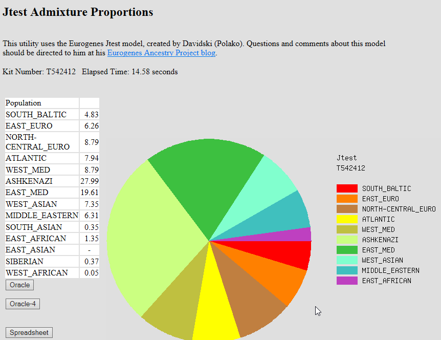 But still, there was something disconcerting about our Jewishness being “confirmed” by a biological test. After all, the reason my grandparents had to leave the towns and villages of their ancestors was because of ethno-nationalism emboldened by a racialized conception of Jewishness as something that exists “in the blood”. The raw memory of this racism made any suggestion of Jewish ethnicity slightly taboo in my family. If I ever mentioned that someone “looked Jewish” my grandmother would respond, “Oh really? And what exactly does a Jew look like?” Yet evidently, this wariness of ethnic categorization didn’t stop my parents from sending swab samples from the inside of their cheeks off to a direct-to-consumer genetic testing company. The idea of having an ancient identity “confirmed” by modern science was too alluring.  Not that they’re alone. As of the beginning of this year, more than 26 million people have taken at-home DNA tests. For most, like my parents, genetic identity is assimilated into an existing life story with relative ease, while for others, the test can unearth family secrets or capsize personal narratives around ethnic heritage. But as these genetic databases grow, genetic identity is re-shaping not only how we understand ourselves, but how we can be identified by others. In the past year, law enforcement has become increasingly adept at using genetic data to solve cold cases; a recent study shows that even if you haven’t taken a test, chances are you can be identified by authorities via genealogical sleuthing. What is perhaps more concerning, though, is how authorities around the world are also beginning to use DNA to not only identify individuals, but to categorize and discriminate against entire groups of people. |
|
|
|
Post by Admin on Aug 12, 2019 23:30:00 GMT
“A very, very long time ago – generations and generations ago – my family consisted of Sephardic Jews,” Ocasio-Cortez said. “The story goes, during the Spanish Inquisition, so many people were forced to convert on the exterior to Catholicism, but on the interior continued to practice their faith and continued to be who they were, even though they were pressured to not be that on the outside world.”  Her family later fled to Puerto Rico to escape persecution, Ocasio-Cortez said. Following the expulsion of non-Christians from Spain in 1492, thousands of Sephardic Jews were forced to convert to Catholicism. Many continued to practice Judaism in secret even after ostensibly converting to Catholicism. Many of these secret Jews, dubbed the “Anusim” (‘Coerced Ones’), emigrated to the Western Hemisphere, settling in colonies across what would become Latin America.  According to Reconectar, an NGO which helps descendants of Anusim reconnect with their Jewish heritage, there are at least 14 to 15 million self-identified ‘Bnei Anusim’ (descendants of Anusim), with as many as 100 million descendants worldwide of Iberian Jews who were forced to convert to Catholicism. “Given the birthrate over the years, studies have estimated the number of descendants of these Jews at anywhere from 100 million to 150 million and even some who claim there are as many as 200 million around the world descended from Spanish and Portuguese Jews,” Reconectar President Ashley Perry told Arutz Sheva. According to the Beit Hatfutsot (Diaspora Museum) in Tel Aviv, Cortez, Ocasio-Cortez’s mother’s maiden name, was a Jewish family name. According to Reconectar, an NGO which helps descendants of Anusim reconnect with their Jewish heritage, there are at least 14 to 15 million self-identified ‘Bnei Anusim’ (descendants of Anusim), with as many as 100 million descendants worldwide of Iberian Jews who were forced to convert to Catholicism. “Given the birthrate over the years, studies have estimated the number of descendants of these Jews at anywhere from 100 million to 150 million and even some who claim there are as many as 200 million around the world descended from Spanish and Portuguese Jews,” Reconectar President Ashley Perry told Arutz Sheva. |
|
|
|
Post by Admin on Aug 13, 2019 18:43:02 GMT
The history of Latin America has involved extensive admixture between Native Americans and people arriving from other continents, particularly Europe and Africa1,2,3. Most genetic studies carried out to date have examined this process mainly in relation to variation in overall Native American, European and Sub-Saharan African ancestry across regions and between individuals2,3,4; with small and geographically-restricted East Asian ancestry also reported5,6,7. In addition, some genetic analyses have sought to detect regional ancestry within the three major continental components, i.e. the sub-continental origins for individuals having contributed to admixture in Latin America. For instance, mtDNA and Y-chromosome data suggest that historical admixture in North West Colombia involved local Native women, and that some immigrant men carried haplogroups common in Jewish populations8. The inference that historical admixture of Latin Americans in specific regions involved Natives with a relatively close genetic affinity to those currently living in the same areas was subsequently supported using genome-wide autosomal data9,10. Recent genome-wide SNP studies (GWAS), partly implementing haplotype-based analyses, have further expanded the notion that the demographic shifts of the last few generations have not entirely erased signals of historical population structure in Latin America6,11,12,13,14,15. A finer characterization of the admixture history of Latin America would benefit from a more extensive sampling across the region, as well as from further methodological improvements (including fully haplotype-based analyses and improved modelling approaches) and a wider survey of reference population samples (from areas potentially contributing to Latin American admixture). 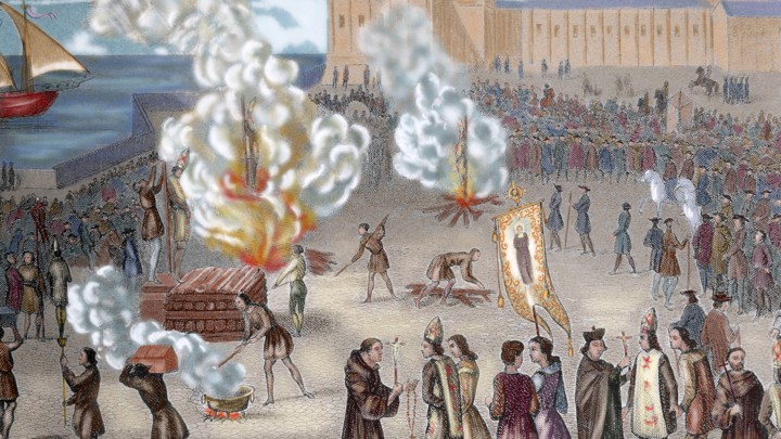 The broad significance of characterizing these fine-grained patterns of human genetic diversity in Latin America is emphasized by the realization that geographically-restricted genetic variation is potentially a key component of the genetic architecture of common human phenotypes, including disease16. Furthermore, studies of regional human genome diversity, and its bearing on phenotypic variation, have so far been strongly biased towards European-derived populations17. The study of populations with non-European ancestry is essential if we are to obtain a more complete picture of human diversity. Latin America represents an advantageous setting in which to examine regional genetic variation and its bearing on human phenotypic diversity18, considering that the extensive admixture resulted in a marked genetic and phenotypic heterogeneity2,3,19. Relative to disease phenotypes, the genetics of physical appearance can be viewed as a model setting with distinct advantages for analyzing patterns of genetic and phenotypic variation. Many physical features are relatively simple to evaluate, show substantial geographic diversity and are highly heritable. We have previously shown that variation at a range of physical features correlates with continental ancestry in Latin Americans19 and have identified genetic variants with specific effects for a number of features20,21,22. 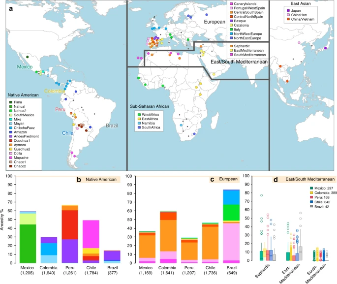 Fig. 1 Reference population samples and SOURCEFIND ancestry estimates for the five Latin American countries examined. a Colored pies and grey dots indicate the approximate geographic location of the 117 reference population samples studied. These samples have been subdivided on the world map into five major bio-geographic regions: Native Americans (38 populations), Europeans (42 populations), East/South Mediterraneans (15 populations), Sub-Saharan Africans (15 populations) and East Asians (7 populations). The coloring of pies represents the proportion of individuals from that population included in one of the 35 reference groups defined using fineSTRUCTURE (these groups are listed in the color-coded insets for each region; Supplementary Fig. 2). The small dark grey dots indicate reference populations not inferred to contribute ancestry to the CANDELA sample. b–d refer to the CANDELA dataset. b, c show, respectively, the average estimated proportion of sub-continental Native American and European ancestry components in individuals with >5% total Native American or European ancestry in each country sampled; the stacked bars are color-coded as for the reference population groups shown in the insets of (a). d shows boxplots of the estimated sub-continental ancestry components for individuals with >5% total Sephardic/East/South Mediterranean ancestry. In this panel colors refer to countries as for the colored country labels shown in (a). Following standard convention for boxplots, the center line denotes the median, the box boundaries represent the first and the third quartiles, and the whiskers range to 1.5 times the inter-quartile range on either side. Outlying points are plotted individually Anthropological studies indicate that Pre-Columbian Native population density varied greatly across the Americas, impacting on the extent of Native American ancestry observed across Latin America2. Native ancestry in the CANDELA sample varies considerably between countries, and we also observe a marked geographic differentiation in sub-continental Native ancestry within each country, with a strong correspondence with the genetic structure of the Native American reference groups (Figs. 1 and 2). Allele-based analyses have previously documented that broad patterns of Native American population structure are detectable in admixed Latin Americans10,14. Our haplotype-based analyses significantly extend these results by enabling the inference of 25 Native American ancestry components across Latin America (Supplementary Fig. 3), which we combined into 16 components for visualization (Figs. 1b and 2a). In Mexicans we find a predominant Nahua sub-component (most prevalent across northern and central Mexico) and two smaller sub-components, one related to Natives of south Mexico and another to Mayans (seen mainly in Mexicans from Yucatan), similar to previous reports14,28. In Peruvians we observe a predominant Quechua component (in central Peru), a sub-component related to Andean-Piedmont Natives (concentrating in Northern Peru) and a smaller Aymara sub-component (seen mostly in Southern Peruvians). In Chileans the predominant Native sub-component is most closely related to the Mapuche from Southern South America, while smaller components, related to those observed in Peruvians, are observed in Northern Chileans. In Colombians Native ancestry is most similar to Chibchan-Paezan Natives from Colombia and lower Central America, particularly in Northwestern Colombians. Other components are most closely related to the Central American Maya and, in Southern Colombians, to the Peruvian Andean Piedmont component. The overlap in Native Ancestry between Peru and neighboring Chile (to the south) and Colombia (to the north) is consistent with the high population density of the Central Andes in pre-Columbian America, possibly associated with major cultural developments in the region (at its peak the Inca Empire extended from southern Colombia to northern Chile29). Finally, Andean-Piedmont ancestry from North-eastern Peru represents the major Native American contribution in the Brazilian sample (Fig. 2; Supplementary Fig. 4). Considering the low Native American ancestry in this sample compared to the other countries sampled (Fig. 1b; most Brazilians examined originate from an area of high recent European immigration19) and the lack of better surrogates for the Native American ancestors of current-day Brazilians (Fig. 1a), this affinity suggests a common ancestral origin between the ancestors of these Brazilians and other populations from the Amazon basin. Our results provide a high-resolution picture of Native variation across the Americas, emphasizing the genetic continuity between pre-Columbian groups and the Native component of present-day admixed populations across the region. |
|

